Section 01 · Definition
What is LLM model routing?
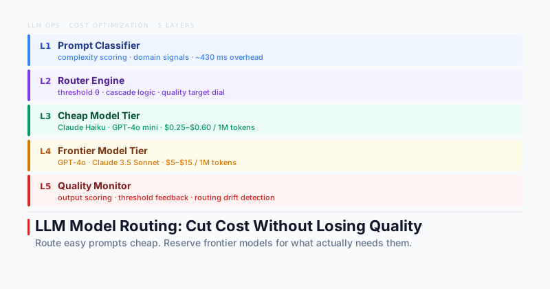
A classification layer that sits in front of your model pool and sends each prompt to the cheapest model capable of answering it adequately.
Quick answer
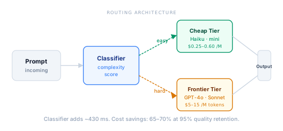
In one sentence: LLM model routing is a classification layer that scores each incoming prompt for complexity, then directs simple requests to cheap, fast models like Claude Haiku or GPT-4o mini and reserves frontier models for the small fraction of queries that genuinely need them.
The economics are stark. Frontier models cost $5 to $15 per million tokens. Cheap models cost $0.25 to $0.60 per million tokens — an order of magnitude less. If you send every request to a frontier model because “it is better,” you are paying 10 to 25 times more than necessary for the half of your traffic that any capable model handles comfortably.
The insight that makes routing practical is that not all queries are equal. “Summarize this in three bullet points” is not the same problem as “Analyze the edge cases in this multistep agentic workflow and flag compliance risks.” A cheap, fast model handles the former without difficulty. Only the latter needs frontier-level reasoning.
The routing classifier bridges the gap. It adds roughly 430 milliseconds to the request path and pays for itself on the first routed call.
Section 02 · Classification
How the classifier works
The classifier runs before your main model call, analyzes the incoming prompt, and assigns a routing decision — typically in under 500 milliseconds.
Classifiers operate on several signal types. Prompt length and structural complexity are the most obvious: longer prompts with nested instructions signal harder tasks. Domain signals — keywords and n-grams associated with tasks that historically required frontier reasoning like code generation, legal analysis, and multipart reasoning — add a second layer.
Conversation context depth also matters. A single-turn factual query behaves very differently from a multi-turn reasoning session where the model needs to track state across several exchanges. Some teams layer in explicit routing rules based on request metadata — user tier, cost budget, or feature flags — so that high-value users always hit the frontier tier regardless of prompt complexity.
RouteLLM, the Berkeley research project, published benchmark data on classifier performance across multiple routing architectures. Their causal LLM and matrix factorization routers achieved strong performance across MMLU, MT-Bench, and the LMSYS Chatbot Arena benchmark. The key finding: the best classifiers add only around 430 milliseconds to total request latency while correctly routing 80 to 90 percent of traffic.
The classifier's output is a routing decision. In its simplest form: route to cheap or route to frontier. In more sophisticated implementations, it produces a probability score that flows into a threshold or cascade strategy.
Good LLM observability is what makes classifier tuning possible in production. Without per-call traces that record which tier each query hit and what quality score it received, you have no feedback loop for adjusting the threshold. Wire observability first, then add routing.
Section 03 · Cost/Quality Dial
The cost/quality tradeoff dial
The relationship between cost savings and quality retention is not a cliff — it is a continuous dial you control through threshold tuning.
Quick answer
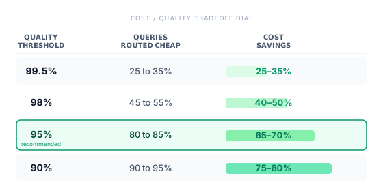
The RouteLLM finding: At a quality threshold of 95 percent, you route 80 to 85 percent of queries to cheaper models for a 65 to 70 percent cost reduction. At 99.5 percent quality retention, you still save 25 to 35 percent by routing easy traffic away from frontier models.
Most teams underestimate this. The tradeoff between cost savings and quality retention is not a cliff — it is a dial you control. RouteLLM benchmarks give a concrete sense of the range across threshold settings.
| Quality threshold | Queries routed cheap | Estimated cost savings |
|---|---|---|
| 99.5% | 25 to 35% | 25 to 35% |
| 98% | 45 to 55% | 40 to 50% |
| 95% | 80 to 85% | 65 to 70% |
| 90% | 90 to 95% | 75 to 80% |
The practical production target for most teams is 95 to 97 percent quality retention, which yields 50 to 65 percent cost savings on routed traffic. The exact numbers shift with your prompt distribution — applications with many short conversational turns and few hard reasoning tasks skew more favorable than the benchmark averages suggest.
One thing worth internalizing: “95 percent frontier quality” is not the same as “5 percent of responses are wrong.” The gap is gradual degradation on the harder tail of your traffic, not catastrophic failure on average queries. The quality monitor is what makes this manageable — you measure the degradation rather than guess at it.
Section 04 · Strategies
Three routing strategies
The literature and production deployments show three main routing patterns. Most teams start with threshold routing and add complexity only when the data justifies it.
Threshold routing
Classify each prompt, assign a complexity score, route cheap if the score is below a threshold θ, route frontier if it is at or above it. Simple to implement and tune. The θ parameter is your quality dial — lower it to save more, raise it to protect quality. This is the right starting point for most teams.
Cascade routing
Send every prompt to the cheap model first. Score the output for quality. If quality clears the threshold, return it directly. If not, escalate to the frontier model and return that response instead. Cascade adds latency for the escalated fraction — two model calls — but is better for safety-critical applications where you want the cheap model to attempt before escalating.
Complexity-aware batching
Classify incoming requests into tiers in real time, batch same-tier requests together, and flush on interval or batch size. Reduces total API calls and works well when your cheap model supports batch inference at further discount. Most useful for async or near-real-time workloads where adding a few seconds of batching delay is acceptable.
Most teams start with threshold routing because it is the simplest to reason about and tune. Cascade routing is worth adding when classifier confidence is noisy — when false negatives on hard prompts are a meaningful risk in your workload and the extra latency is acceptable.
Section 05 · Optimization Stack
Routing in the LLM cost optimization stack
Routing is one of four major levers for LLM cost reduction. Pairing them compounds the savings — the levers attack the cost curve from different angles.
| Lever | Typical savings | Complexity | Implement when |
|---|---|---|---|
| Semantic caching | 30 to 70% | Low | Always — implement first |
| Prompt compaction | 20 to 50% | Low to medium | Multi-turn agents with long history |
| Model routing | 25 to 70% | Medium | $3k+ monthly LLM spend |
| Batch inference | 20 to 50% | Medium | Async workloads: reports, embeddings |
Routing and caching compose well. Cache hits arrive before the router sees them, reducing the total volume the classifier must process. The router then handles cache misses. Together they can push effective cost per query down 70 to 80 percent versus a naive all-frontier setup.
For teams running agent workflows, prompt compaction and routing address the token budget from different angles and should be considered together. The LLM inference cost optimization playbook covers implementation priority and sequencing across all four levers, with concrete benchmarks from production deployments.
Section 06 · Decision Guide
When routing is worth the added complexity
Routing adds engineering and operational overhead: a classifier to build or procure, thresholds to tune, quality monitoring to wire in, and routing drift to watch for over time.
Quick answer
The break-even signal: At roughly $3,000 to $5,000 per month in model spend, the engineering cost of building and tuning a router typically pays back within a quarter. Below that threshold, semantic caching alone gives better return per engineering hour.
Monthly spend exceeds $3,000 to $5,000
Below this threshold, semantic caching and prompt compaction give better return per engineering hour. Above it, the classifier build cost and ongoing tuning pay back within a quarter at typical savings rates.
Your prompt distribution is bimodal
Log 1,000 consecutive production queries, run them through a classifier offline, and measure the quality gap at different threshold settings. If the distribution shows a large easy tail, routing is worth building. If the prompts are uniformly complex, the classifier will rarely route anything and the overhead is wasted.
You have a quality monitoring baseline
Routing without observability is routing blind. You need per-call traces that record which tier each query hit, what quality score it received, and whether users accepted or rejected the response. Without this feedback loop, threshold tuning is guesswork.
Skip routing: uniformly hard use cases
Code review on large codebases, adversarial red-teaming, complex legal analysis — there is no cheap tier that clears quality gates. The classifier adds latency for nothing. Spend the engineering time on prompt compaction instead.
Skip routing: reproducibility requirements
Certain compliance workflows require deterministic outputs across 100 percent of requests. Routing introduces model nondeterminism even on easy queries because different model families produce structurally different outputs for the same prompt.
If you are unsure whether your distribution is bimodal, run the offline experiment before committing to building a router. The data will tell you whether routing is worth adding — and what threshold setting to start with — before you write a line of production code.
If routing is the right fit, the AI Systems Architecture service covers the full design: classifier selection, threshold calibration, quality monitoring integration, and ongoing drift detection as your prompt distribution evolves.